Contrasts in Multilevel/Mixed Models
Regression (and multilevel/mixed models) gives an estimate of the effect of an independent variable on the dependent variable.
When estimating the effect of a categorical independent variable, the mixed model will estimate the effect of each of its levels, and tell us if each effect is significantly different from zero. This is useful information, however, most researcher will be interested in knowing if the levels of the independent variable differ from each other.
Taking the sleepstudy example again, and consider Days as a categorical rather than a continous variable, and ask the question does Reaction on day 1 differ from Reaction on day 2/3/4 etc?
Implementing the formula
The first step is to change the format of Days from continuous to factor. Second, when running the model, we will remove the fixed intercept, by subtracting 1 from the formula. This subtraction does not change the result but will make the successive operations a little easier as it provides the complete display of all the factor levels.
# install.packages("lmerTest")
# install.packages("knitr")
# install.packages("multcomp")
# install.packages("dplyr")
# install.packages("ggplot2")
data("sleepstudy")
# Load packages
packs <- c("lmerTest", "knitr", "multcomp", "dplyr", "ggplot2")
lapply(packs, require, character.only = TRUE)
This is the data as we already have visualised it before:
kable(head(sleepstudy))
| Reaction | Days | Subject |
|---|---|---|
| 249.5600 | 0 | 308 |
| 258.7047 | 1 | 308 |
| 250.8006 | 2 | 308 |
| 321.4398 | 3 | 308 |
| 356.8519 | 4 | 308 |
| 414.6901 | 5 | 308 |
But we will change the format of Days to categorical, transforming it into a type of variable that is called factor in R. The levels of a factor are its possible values, in this case, Day 0, 1, 2, 3, 4 etc.
# Change the data type of Days from number (continous) to factor (categorical)
sleepstudy$Days <- factor(as.character(sleepstudy$Days),
                          levels = unique(sleepstudy$Days))
levels(sleepstudy$Days)
[1] “0” “1” “2” “3” “4” “5” “6” “7” “8” “9”
And re-fit the model:
# Fit the model
m <- lmer(Reaction ~ Days - 1 + ( 1 | Subject), data=sleepstudy)
kable(coef(summary(m)))
| Estimate | Std. Error | df | t value | P-value | |
|---|---|---|---|---|---|
| Days0 | 256.6518 | 11.45778 | 41.98297 | 22.39978 | <2e-16 *** |
| Days1 | 264.4958 | 11.45778 | 41.98297 | 23.08438 | <2e-16 *** |
| Days2 | 265.3619 | 11.45778 | 41.98297 | 23.15997 | <2e-16 *** |
| Days3 | 282.9920 | 11.45778 | 41.98297 | 24.69867 | <2e-16 *** |
| Days4 | 288.6494 | 11.45778 | 41.98297 | 25.19243 | <2e-16 *** |
| Days5 | 308.5185 | 11.45778 | 41.98297 | 26.92654 | <2e-16 *** |
| Days6 | 312.1783 | 11.45778 | 41.98297 | 27.24596 | <2e-16 *** |
| Days7 | 318.7506 | 11.45778 | 41.98297 | 27.81957 | <2e-16 *** |
| Days8 | 336.6295 | 11.45778 | 41.98297 | 29.37999 | <2e-16 *** |
| Days9 | 350.8512 | 11.45778 | 41.98297 | 30.62122 | <2e-16 *** |
The output shows that each Day separately has a very significant effect on Reaction.
But do the Days actually differ from each other? The easiest way of comparing factors between each other is to choose a reference level. In this example, we will assume the first day of the experiment, Day 1, as a reference, and compare all the other days to Day 1.
Building the Contrasts Matrix
First, we need to compute all the combinations of the levels of the factor Day in a Contrasts Matrix:
group <- paste0(sleepstudy$Days)
group <- aggregate(model.matrix(m) ~ group, FUN=mean)
# group
rownames(group) <- group$group
(group <- group[,-1])
kable(group)
| Days0 | Days1 | Days2 | Days3 | Days4 | Days5 | Days6 | Days7 | Days8 | Days9 | |
|---|---|---|---|---|---|---|---|---|---|---|
| 0 | 1 | 0 | 0 | 0 | 0 | 0 | 0 | 0 | 0 | 0 |
| 1 | 0 | 1 | 0 | 0 | 0 | 0 | 0 | 0 | 0 | 0 |
| 2 | 0 | 0 | 1 | 0 | 0 | 0 | 0 | 0 | 0 | 0 |
| 3 | 0 | 0 | 0 | 1 | 0 | 0 | 0 | 0 | 0 | 0 |
| 4 | 0 | 0 | 0 | 0 | 1 | 0 | 0 | 0 | 0 | 0 |
| 5 | 0 | 0 | 0 | 0 | 0 | 1 | 0 | 0 | 0 | 0 |
| 6 | 0 | 0 | 0 | 0 | 0 | 0 | 1 | 0 | 0 | 0 |
| 7 | 0 | 0 | 0 | 0 | 0 | 0 | 0 | 1 | 0 | 0 |
| 8 | 0 | 0 | 0 | 0 | 0 | 0 | 0 | 0 | 1 | 0 |
| 9 | 0 | 0 | 0 | 0 | 0 | 0 | 0 | 0 | 0 | 1 |
The 1s specify when a level is active - given that we only have one factor, when one level is active (1), all the others are inactive (0). The matrix becomes more complicated if you have more than one factor. We can now specify the custom contrasts we want to compute between the levels, in this case, all levels against Day 1 of the experiment:
contrasts <- rbind(group["1",] - group["0",],
                   group["1",] - group["2",],
                   group["1",] - group["3",],
                   group["1",] - group["4",],
                   group["1",] - group["5",],
                   group["1",] - group["6",],
                   group["1",] - group["7",],
                   group["1",] - group["8",],
                   group["1",] - group["9",])
kable(contrasts)
| Days0 | Days1 | Days2 | Days3 | Days4 | Days5 | Days6 | Days7 | Days8 | Days9 | |
|---|---|---|---|---|---|---|---|---|---|---|
| 1 | -1 | 1 | 0 | 0 | 0 | 0 | 0 | 0 | 0 | 0 |
| 11 | 0 | 1 | -1 | 0 | 0 | 0 | 0 | 0 | 0 | 0 |
| 12 | 0 | 1 | 0 | -1 | 0 | 0 | 0 | 0 | 0 | 0 |
| 13 | 0 | 1 | 0 | 0 | -1 | 0 | 0 | 0 | 0 | 0 |
| 14 | 0 | 1 | 0 | 0 | 0 | -1 | 0 | 0 | 0 | 0 |
| 15 | 0 | 1 | 0 | 0 | 0 | 0 | -1 | 0 | 0 | 0 |
| 16 | 0 | 1 | 0 | 0 | 0 | 0 | 0 | -1 | 0 | 0 |
| 17 | 0 | 1 | 0 | 0 | 0 | 0 | 0 | 0 | -1 | 0 |
| 18 | 0 | 1 | 0 | 0 | 0 | 0 | 0 | 0 | 0 | -1 |
Now the matrix specifies couples of contrasts that we want to estimate from the model.
Extracting the contrasts from the model
For extracting the contrasts from the model, we are going to use the glht function from the multcomp package.
library(multcomp)

# Format the matrix for better readibility
contrast.matrix <- rbind("Day 1 versus Day 0"=as.numeric(contrasts[1,]),
                         "Day 1 versus Day 2"=as.numeric(contrasts[2,]),
                         "Day 1 versus Day 3"=as.numeric(contrasts[3,]),
                         "Day 1 versus Day 4"=as.numeric(contrasts[4,]),
                         "Day 1 versus Day 5"=as.numeric(contrasts[5,]),
                         "Day 1 versus Day 6"=as.numeric(contrasts[6,]),
                         "Day 1 versus Day 7"=as.numeric(contrasts[7,]),
                         "Day 1 versus Day 8"=as.numeric(contrasts[8,]),
                         "Day 1 versus Day 9"=as.numeric(contrasts[9,]))

comparisons <- summary(glht(m, contrast.matrix))

comparisons
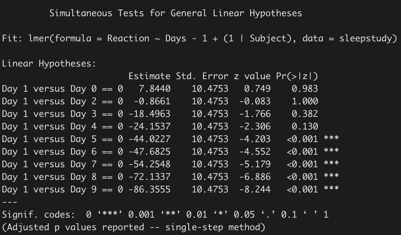
The output shows that Reaction is not significantly different from baseline (Day 0) on Day 1. Also, Reaction only starts to differ from baseline since Day 5, and the difference grows progressively until Day 9.
Let’s format the results of the contrasts test into a table:
pq <- comparisons$test

mtests <- data.frame(pq$coefficients, pq$sigma, pq$tstat, pq$pvalues)
error <- attr(pq$pvalues, "error")
pname <- switch(comparisons$alternativ,
                less = paste("Pr(<",
                             ifelse(comparisons$df ==0, "z", "t"), ")",
                             sep = ""),
                 greater = paste("Pr(>",
                                 ifelse(comparisons$df == 0, "z", "t"), ")",
                                 sep = ""),
                 two.sided = paste("Pr(>|",
                                   ifelse(comparisons$df == 0, "z", "t"), "|)"
                                   , sep = ""))
colnames(mtests) <- c("Estimate", "Std.Error",
                      ifelse(comparisons$df ==0, "zvalue", "tvalue"), pname)

mtests <- mtests %>%
  tibble::rownames_to_column("Comparison") %>%
  mutate(`Pr(>|z|)`=ifelse(`Pr(>|z|)`< 0.001,
                           "< 0.001",
                           ifelse(`Pr(>|z|)` < 0.01,
                                  "< 0.01",
                                  ifelse(`Pr(>|z|)` < 0.05,
                                         "< 0.05",
                                         paste(round(`Pr(>|z|)`,
                                                     4)))))) %>%
  mutate_if(is.numeric, funs(round(.,
                                   digits=2)))
kable(mtests)
| Estimate | Std.Error | zvalue | Pr(>|z|) | |
|---|---|---|---|---|
| Day 1 versus Day 0 | 7.8439500 | 10.47531 | 0.7488038 | 0.9827613 |
| Day 1 versus Day 2 | -0.8661444 | 10.47531 | -0.0826844 | 1.0000000 |
| Day 1 versus Day 3 | -18.4962556 | 10.47531 | -1.7657006 | 0.3815733 |
| Day 1 versus Day 4 | -24.1536667 | 10.47531 | -2.3057718 | 0.1301341 |
| Day 1 versus Day 5 | -44.0227000 | 10.47531 | -4.2025213 | 0.0002050 |
| Day 1 versus Day 6 | -47.6825000 | 10.47531 | -4.5518953 | 0.0000436 |
| Day 1 versus Day 7 | -54.2548278 | 10.47531 | -5.1793068 | 0.0000019 |
| Day 1 versus Day 8 | -72.1337500 | 10.47531 | -6.8860751 | 0.0000000 |
| Day 1 versus Day 9 | -86.3554667 | 10.47531 | -8.2437171 | 0.0000000 |
Next Steps
Contrasts can be customised depending on the research question at hand, and much more complicated contrasts matrix are often needed.
Another scenario when this procedure may turn out useful is when an interaction is present. In that case, the contrasts matrix will indicate the combination between two different factors. We will explore an example with an interaction in the next post.
Teresa Del Bianco
Postdoctoral Researcher
Scientist researching brain and child development and neurodiversity.