Linear regression on transformed variables
In the previous post, we examined the relationship between a dependent variable and a couple of independent variables from the example ‘Chickweight’ dataset.
Upon checking of the assumptions, we found that the data did not follow a linear pattern, and residuals were heteroscedastic.
#install.packages("ggplot2")
#install.packages("knitr")
library(ggplot2)
data("ChickWeight")
knitr::kable(head(ChickWeight))
| weight | Time | Chick | Diet |
|---|---|---|---|
| 42 | 0 | 1 | 1 |
| 51 | 2 | 1 | 1 |
| 59 | 4 | 1 | 1 |
| 64 | 6 | 1 | 1 |
| 76 | 8 | 1 | 1 |
| 93 | 10 | 1 | 1 |
For addressing both of this problems, we can attempt a non-linear transformation of the dependent variable (Weight), and the problematic independent variable (Time)
For the heteroscedacity problem, we may choose a “concave” function, such as the logarithmic transformation.
lrlog <- lm(log(weight) ~ Time + Diet, data = ChickWeight)

ggplot(data=ChickWeight,
       aes(x=predict(lrlog), y=resid(lrlog))) +
  geom_point(size = 3, col = "red", alpha = 0.6) +
  geom_abline(slope = 0,
              intercept = 0,
              col = "gray") +
  labs(x = "Fitted Values", y = "Residuals",
       title = "Residuals vs Fitted",
       subtitle = "Log Transformation") +
  coord_fixed()

The pattern has changed but it is still heteroscedastic; we may also attempt to transform Time to a cubic function. This can be done by using the I function, e.g., I(Time^2) + I(Time^3). However, this method introduces a correlation between the two new terms. Therefore, we could use the function poly, that generates orthogonal transformations, i.e., not correlated between each other.
lrlogcub <- lm(log(weight) ~ poly(Time,3) + Diet, data = ChickWeight)

ggplot(data=ChickWeight,
       aes(x=predict(lrlogcub), y=resid(lrlogcub))) +
  geom_point(size = 3, col = "red", alpha = 0.6) +
  geom_abline(slope = 0,
              intercept = 0,
              col = "gray") +
  labs(x = "Fitted Values", y = "Residuals",
       title = "Residuals vs Fitted",
       subtitle = "Log and Cubic Transformation") +
  coord_fixed()
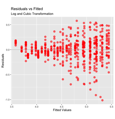
Adding a cubic transformation of time seems to improve the fit. The points that lay well below the average may be outliers - that are far more visible now (although the treatment of outliers should be pondered carefully).
Let’s check if we get a similar result as before.
knitr::kable(coef(summary(lrlogcub)))
| Estimate | Std. Error | t value | Pr(>|t|) | |
|---|---|---|---|---|
| (Intercept) | 4.5091139 | 0.0147902 | 304.8719977 | 0.0000000 |
| poly(Time, 3)1 | 12.5890056 | 0.2194134 | 57.3757310 | 0.0000000 |
| poly(Time, 3)2 | -1.5253665 | 0.2193305 | -6.9546486 | 0.0000000 |
| poly(Time, 3)3 | -0.1704505 | 0.2193259 | -0.7771562 | 0.4373885 |
| Diet2 | 0.1199428 | 0.0248970 | 4.8175605 | 0.0000019 |
| Diet3 | 0.2474644 | 0.0248970 | 9.9395248 | 0.0000000 |
| Diet4 | 0.2457223 | 0.0250289 | 9.8175523 | 0.0000000 |
The output is similar, although, since we transformed the dependent variable, all the Estimates are now on the logarithmic scale (so they can be back-transformed with exp). Also, we have 3 distinct Time variables, each describing a particular pattern that could be attributed to Time.
Overall, we could say that the result did not change much, as we still have a significant effect of Time and of each of the diets. Also, the extent of effectiveness of the Diets (4 is the best, 2 is the least effective) is preserved. Therefore, we could use this approach - that is a little more difficult to interpret and communicate to others - to validate our previous analysis.
Collinearity
Another aspect that is worth checking is collinearity, or correlation, between the independent variables. If the independent variables are correlated between each other, it might introduce a bias in the regression. If that is the case, the effect of the two variables cannot be disentangled and a different approach should be taken (for example, the variables should be combined with a Factor Analysis).
Normally, one could simply plot the independent variables one against the other with the function plot, and calculating the correlation coefficient with cor.
However, in this case, it does not make much of a sense because the variable Diet is categorical. We can have a sense of the association between the two independent variables by regressing the two and looking at the correlation between the residuals and the data - as measured by the squared root of the R-Squared.
lr_coll <- lm(Time ~ Diet, data = ChickWeight)
rsq <- summary(lr_coll)$r.squared
sqrt(rsq)
0.02882599
The squared root of R-Squared is very small, so we may conclude that the collinearity between the two independent variable is negligible.
Teresa Del Bianco
Postdoctoral Researcher
Scientist researching brain and child development and neurodiversity.